Near field speaker measurement using SoundEasy

How to make a near field measurement?

Making a near field speaker measurement should be child’s play, if you have done far field before. This measuring technique is very useful for measuring the very low frequencies. As a result, when we are talking about near field, woofers and bass reflex ports are the prime candidates. Furthermore, this method let’s us make anechoic measurements, without an anechoic chamber. Long wavelength reflections are especially tricky indoors, and the near field method makes life a whole lot easier. Make sure you read the far field measurement article before you start this one.

Near field speaker measurement theory

Basically, you place the microphone as close as you can to the center of the speaker, and take a measurement. Being so close to the speaker, it negates all reflections, diffraction etc. The only downside is that the measurement is valid up to a certain point. This means that the low frequencies are measured accurately, but as you go up the frequency spectrum, you reach a point when the measurement is invalid.

This point is determined by the size of the speaker. f_max = 10950 / D , where D = the diameter of the speaker in centimeters. We will be measuring a SEAS CA 18 RNX (Amazon affiliate paid link) in a 15 liter bass reflex box. The diameter of the speaker is 13.16 cm, so f_max = 10950 / 13.16 = 832 Hz. This means our near field speaker measurement will be accurate 20 Hz – 832 Hz.

Near field port measurement theory

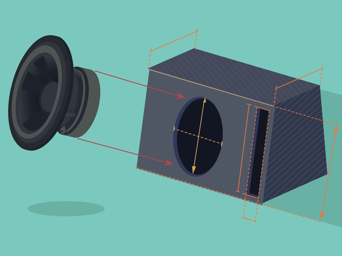
Measuring the port is done in a similar fashion. You place the microphone in the center of the port, flush (don’t stick it in). There is no more talk about dimensions and how high you can go in frequency, because the port will definitely have a tuning frequency under 100 Hz. However, in almost all cases there will be a size mismatch between the speaker and the port. The port will be smaller. Very rarely they are the same size. As a result, before we add the responses together, we need to scale them according to their size.

To do so, you need to calculate the area of the speaker and the area of the port. Our enclosure uses a 68 mm port (3.4 cm radius).

• The area of the speaker should be in the spec sheet. Otherwise, calculate it. Effective piston area = 136 cm².
• The area of the port is πR² = 3.14 * 3.4 *3.4 = 36.30 cm².

The formula for calculating the scaling is :  20 * log (A_p / A_s)^0.5 , where :

• A_p = area of the port.
• A_s = area of the speaker.

So, in our case, the scaling is 20 * log(36.30/136)^0.5 = 20 * log(0.267)^0.5 = 20 * log(0.5166) = 20 * (-0.2868) = -5.7 dB. In conclusion, the response of the port needs to be scaled down by 5.7 dB. In almost all cases this will be a negative number, since the ports are smaller in size compared to the speaker.

Baffle step correction

When making a near field speaker measurement, the microphone is placed very close to the speaker. As a result, the microphone doesn’t pick up the boost of the baffle. Depending on the size of the baffle, certain frequencies are boosted. First, make sure you have entered the size of your speaker in the Driver Editor.

Then, go to Enclosure Tools -> Front Baffle Design / Diffraction.

Here we need to model our enclosure, and the position of the driver on the baffle. The size of my baffle is 23 cm wide by 33 cm tall. Make sure to check the position of the center of the driver, because we need to model that also. The microphone position will coincide with the center of the speaker position.

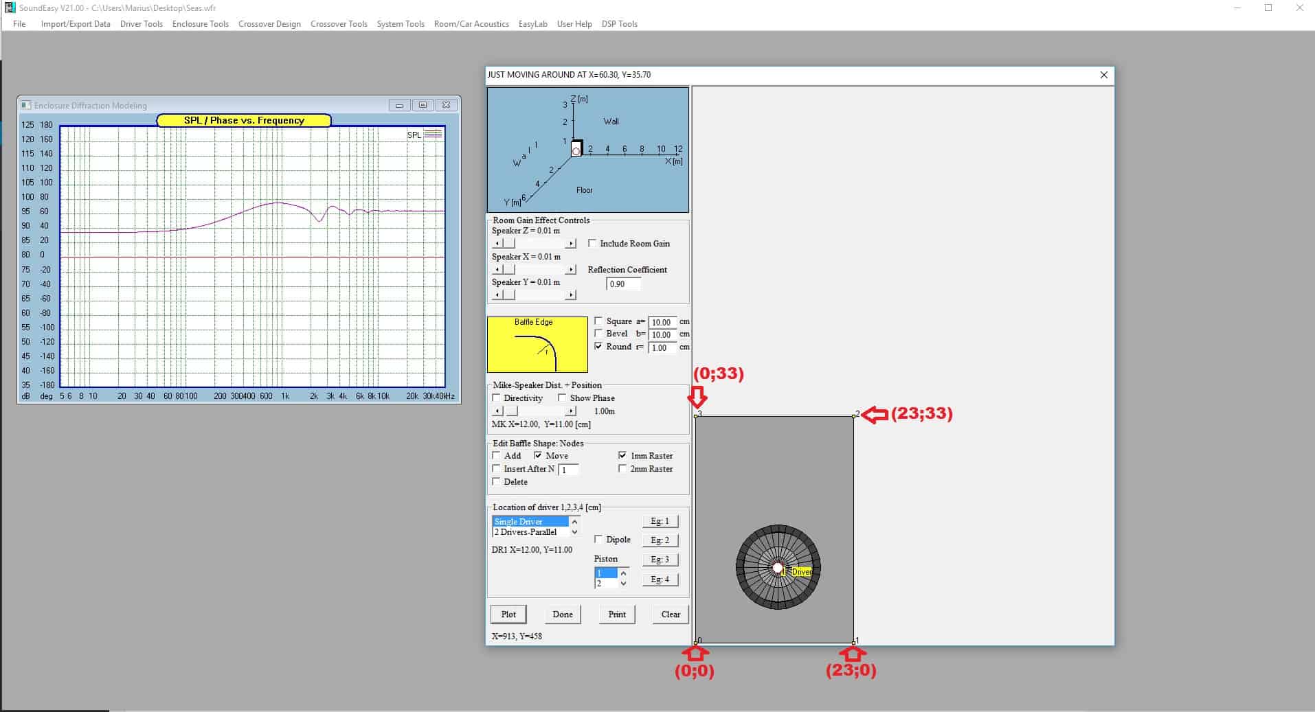
• Leave the room gain effects alone.
• If your baffle edge is square, leave it like that. Mine is round, with 1 cm radius.
• Leave the mic distance at 1 meter and drag it to its position. The mic is the red circle, and place it at the same position with the center of the speaker.
• Depending on the shape oh the baffle you can add or delete nodes. Otherwise, leave the “Move” box checked, so you can move the nodes in the sketch.
• Move the nodes to the correct positions, depending on the size of your baffle (mine is 23 x 33 cm). If you can lower your mouse’s sensitivity, it helps.
• Place the speaker at the correct position (it should match the mic position).
• Press Plot button.

Speaker near field measurement

Go ahead and place the microphone very close to the center of the speaker.

Do the exact same steps as in the far field measurement article. The only difference is that the window must be negated. This near field speaker measurement doesn’t suffer from reflections and such. There is no option to turn off the window, so the only thing left to do is to set a big enough window that it doesn’t even matter. I go for 500 ms. Now, all that’s left is to set the levels. Just like before, increase the volume in small steps and check the levels each time, until you get a satisfactory result. Take extra caution, as the microphone is almost touching the speaker. As a result, even the faintest sound will sound loud. If you hear the speaker hitting the mic, move it back a little.

How to design loudspeakers - video courses

Acoustics 101 : Speaker design basics and enclosure design

Acoustics 201 : Loudspeaker measurements

Loudspeaker engineering : How to design speaker crossovers

Read more and sign up

I trust you are already in the Easy Lab -> Digital MLS menu.

Run MLS and then click the IR -> SPL button so the graph shows up.

Extra : Tuning frequency of bass reflex box

It has nothing to do with our frequency response measurement, but when you are doing a near field speaker measurement, which is placed in a bass reflex box, a dip will show up. This dip corresponds to the resonant frequency of the enclosure. This happens because at the tuning frequency of the box, the port (Amazon affiliate paid link) does all the work and the speaker barely moves. For this reason, there will be a dip in the response curve. It seems that my enclosure is tuned at 51 Hz.

Now go ahead and click the Post Processing tab.

Click the SPL to Buffer 1. What this basically does, is saving the response in the first slot. We have 5 available slots on which we can save response curves. Then, we can manipulate them how we want, add them, subtract, etc. Optionally, you can click the “Show Curve” check box, so you can see the response of the corresponding slot. For now, we leave the response alone, as we also need the port response.

Port near field measurement

Go ahead and place the microphone in the center of the port, flush with the baffle.

Now, head back to the MLS tab, click the Clear SPL / Zin button, and run another frequency measurement. Keep the same settings as before. Don’t alter the output volume, or the amplifier volume. It should look something like this :

After the measurement is finished, go back to the Post Processing tab. Save it to the 2nd slot, and it should look something like this :

Combining the 2 curves

To get the complete low end response, we have to combine the 2 response curves (speaker + port).

Step 1 : Scale the port response

As we calculated beforehand, the response of the port needs to scaled down by 5.7 dB.

Port response is saved to Buffer 2, so we are going to add -5.7 dB to it.

Step 2 : Add the 2 responses together

Now that the curves are scaled to the same level, we can add them up.

• Check the boxes under the “+” sign, next to each curve you want to add up. The minus side is for subtracting (not our case).
• Click Execute Above -> Master Buffer. This will add (or subtract) all the curves we checked above to the Master Buffer. The Master Buffer is essentially Slot 6.
• Copy the Master Buffer to Buffer slot 3. Now the combined response shows on the graph.

Step 3 : Baffle step correction

Now that we finished combining the 2 response curves, we need to apply the baffle step correction. First, make sure that the size of your speaker is set in the “Driver Tools -> Driver Editor”. Secondly, we have to design the baffle in the baffle design editor, but we already did that.

Click the “Add Diffraction to” Buffer 3 button, and this should complete our near field speaker measurement.

Conclusion

The near field speaker measurement has concluded, and now we have a frequency response which is valid up until 800 Hz. We can use this curve to splice it with the far-field curve, and get a full frequency response graph. But that is for a future article.

References

1. Image source : link.